Analysis of a Non-Small Cell Lung Cancer Dataset
lung_analysis.RmdIntroduction
In this vignette, we will demonstrate how to use the
spagg package to aggregate multiple spatial summary
statistics estimated across several regions-of-interest (ROIs) taken
from the same tissue sample, such as from a tumor. We may possess data
for these samples from multiplexed immunofluorescence imaging or spatial
proteomics imaging platforms, which yields spatial information on the
cells residing in the tissue.
# Loading in packages
library(spagg)
library(dplyr)
library(magrittr)
library(spatstat)
library(ggplot2)
library(tidyr)
library(cowplot)
Let’s consider using spagg to analyze a multiplexed
immunohistochemistry (mIHC) dataset generated from a non-small cell lung
cancer study by Johnson et al. (2021). We
will examine the spatial distribution of CD4 T cells and study its
association with major histocompatibility complex II (MHCII) status, a
binary tumor-level label. We will use Ripley’s K to characterize the
spatial colocalization of CD4+ T cells and tumor cells.
Since this study captured multiple ROIs per tumor sample we need a
way of handling multiple estimates of Ripley’s K for each sample.
spagg provides several ways of doing so.
Downloading the Data
First, let’s load in the data we will use. This dataset will be
downloaded from http://juliawrobel.com/MI_tutorial/MI_Data.html but is
also available from the VectraPolarisData R package (Wrobel and Ghosh (2022)). For the purposes of
this illustration, we do some basic tidying of the data prior to
analysis. The steps to this are similar to those given in the link given
above. These steps are shown below.
# Load in the data
load(url("http://juliawrobel.com/MI_tutorial/Data/lung.RDA"))

# Label the immune cell types
lung_df <- lung_df %>%
  mutate(type = case_when(
    phenotype_cd14 == "CD14+" ~ "CD14+ cell",
    phenotype_cd19 == "CD19+" ~ "CD19+ B cell",
    phenotype_cd4 == "CD4+" ~ "CD4+ T cell",
    phenotype_cd8 == "CD8+" ~ "CD8+ T cell",
    phenotype_other == "Other+" ~ "Other",
    phenotype_ck == "CK+" ~ "Tumor"
  ))

# Add a column indicating if a sample has >=5% MHCII+ tumor cells
lung_df <- lung_df %>%
  dplyr::group_by(patient_id) %>%
  dplyr::mutate(mhcII_high = as.numeric(mhcII_status == "high"))

# Change colnames
colnames(lung_df)[colnames(lung_df) == "patient_id"] <- "PID"

# Add a PID column
colnames(lung_df)[colnames(lung_df) == "image_id"] <- "id"

# Filter to just cells detected within the tumor
lung_df_tumor <- lung_df %>% filter(tissue_category == "Tumor")

# Remove grouping
lung_df_tumor <- lung_df_tumor %>% dplyr::ungroup()

# Remove NA types
lung_df_tumor <- lung_df_tumor %>% filter(!is.na(type))

# Show the first few rows of the data
head(lung_df_tumor)
#> # A tibble: 6 × 39
#>   id              PID   cell_id     x     y gender mhcII_status age_at_diagnosis
#>   <chr>           <chr>   <dbl> <dbl> <dbl> <chr>  <chr>                   <dbl>
#> 1 #01 0-889-121 … #01 …       5  453    2.5 F      low                        85
#> 2 #01 0-889-121 … #01 …       6  463    2.5 F      low                        85
#> 3 #01 0-889-121 … #01 …      11  464    8.5 F      low                        85
#> 4 #01 0-889-121 … #01 …      12  538   10   F      low                        85
#> 5 #01 0-889-121 … #01 …      21  522   20.5 F      low                        85
#> 6 #01 0-889-121 … #01 …      22  566.  25   F      low                        85
#> # ℹ 31 more variables: stage_at_diagnosis <chr>, stage_numeric <dbl>,
#> #   pack_years <dbl>, survival_days <dbl>, survival_status <dbl>,
#> #   cause_of_death <chr>, adjuvant_therapy <chr>,
#> #   time_to_recurrence_days <dbl>, recurrence_or_lung_ca_death <dbl>,
#> #   tissue_category <chr>, cd19 <dbl>, cd3 <dbl>, cd14 <dbl>, cd8 <dbl>,
#> #   hladr <dbl>, ck <dbl>, dapi <dbl>, entire_cell_axis_ratio <dbl>,
#> #   entire_cell_major_axis <dbl>, entire_cell_minor_axis <dbl>, …
We first start by plotting the ROIs for an example image. Consider
the first sample, PID=#01 0-889-121 which has five ROIs. We
plot the cells in each of these ROIs below.
# Select the first sample
example <- lung_df %>% dplyr::filter(PID == "#01 0-889-121")

# Plot each of the ROIs and save in a list
plot.list <- lapply(1:5, function(i) list())

for (id.i in unique(example$id)) {

  # Subset
  example.id <- example %>% dplyr::filter(id == id.i)

  # ROI number
  roi <- which(unique(example$id) %in% id.i)

  # Plot
  pp <- example.id %>%
    dplyr::filter(!is.na(type)) %>%
    ggplot(aes(x = x, y = y, color = type)) +
    geom_point() +
    theme_bw() +
    ggtitle(paste0("ROI ", roi)) +
    labs(color = "Cell Type")

  # Save
  plot.list[[roi]] <- pp
}

# Construct the full plot
cowplot::plot_grid(plot.list[[1]], plot.list[[2]],
                   plot.list[[3]], plot.list[[4]],
                   plot.list[[5]], nrow = 3, ncol = 2)
As discussed under the Getting Started vignette, this
can be a helpful exercise to examine how the spatial distribution of
cells varies across ROIs. Notice the varying spatial arrangements of
CD4+ T cells (green) and tumor cells (pink) across ROIs in
particular.
Weighted Aggregations
We first consider the weighted aggregation approaches to handling
multiple ROIs. We introduce the formulations of these aggregations
provided in spagg below:
(Diggle, Lange, and Beneš (1991)), (Baddeley et al. (1993)), and (Landau, Rabe-Hesketh, and Everall (2004)) were each proposed as approaches to aggregating replicated Ripley’s K statistics.
We will estimate Ripley’s K for on each ROI. Note this may take several seconds (up to 1 minute) to run.
# Set the radius
r <- 20

# Save the image IDs
ids <- unique(lung_df_tumor$id)

# Initialize a data.frame to store the results for each ROI
results <- lung_df_tumor %>%
  dplyr::select(PID, id) %>%
  dplyr::distinct() %>%
  dplyr::mutate(spatial = NA,
                npoints = NA,
                area = NA)

# Iterate through the ROIs (this will take a few seconds)
for (i in 1:length(ids)) {

 # Save the ith image
 image.i <- lung_df_tumor %>%
   dplyr::filter(id == ids[i]) %>%
   dplyr::select(x, y, type) %>%
   dplyr::mutate(type = factor(type))

   # Convert to a point process object
   w <- spatstat.geom::convexhull.xy(image.i$x, image.i$y)
   image.i.subset <- image.i %>% dplyr::filter(type %in% c("CD4+ T cell", "Tumor"))
   image.i.subset$type <- droplevels(image.i.subset$type) # Remove unneeded cell types
   image.ppp <- spatstat.geom::as.ppp(image.i.subset, W = w)

   # Check if this image has sufficient numbers of both cell types
   if (length(table(image.ppp$marks)) == 2) {
     # Compute Kest
     Ki <- spatstat.explore::Kcross(image.ppp, i = "CD4+ T cell", j = "Tumor", r = 0:r, nlarge = 10000)

     # Calculate the number of points
     npoints.i <- spatstat.geom::npoints(image.ppp)

     # Calculate the area
     area.i <- spatstat.geom::area(image.ppp)

     # Save the results
     results[results$id == ids[i],]$spatial <- Ki$iso[r+1]
     results[results$id == ids[i],]$npoints <- npoints.i
     results[results$id == ids[i],]$area <- area.i
   }
}

# View the first few rows
head(results)
#> # A tibble: 6 × 5
#>   PID           id                                  spatial npoints    area
#>   <chr>         <chr>                                 <dbl>   <int>   <dbl>
#> 1 #01 0-889-121 #01 0-889-121 P44_[40864,18015].im3   1049.    1439 301361.
#> 2 #01 0-889-121 #01 0-889-121 P44_[42689,19214].im3   1083.    1124 285454.
#> 3 #01 0-889-121 #01 0-889-121 P44_[42806,16718].im3   1429.    1479 332974.
#> 4 #01 0-889-121 #01 0-889-121 P44_[44311,17766].im3    946.    2726 333936.
#> 5 #01 0-889-121 #01 0-889-121 P44_[45366,16647].im3   1856.    1366 333376.
#> 6 #02 1-037-393 #02 1-037-393 P44_[56576,16907].im3     NA       NA     NA
Note that some images had too few CD4+ T cells to compute Ripley’s K. For these images, the resulting spatial summary statistic, area, and number of points defaults to NA. We will remove these images for the subsequent analysis.
We can now visualize the distribution of the spatial summaries within each image as an illustration of the variation in spatial distribution of tumor and CD4+ T cells across ROIs.
# Remove NAs
results <- results[!is.na(results$spatial),]

# Visualize the distribution of spatial summaries within each sample
results %>%
  dplyr::mutate(PID = factor(PID)) %>%
  ggplot(aes(x = PID, y = spatial, group = PID)) +
  geom_boxplot() +
  theme_bw() +
   theme(axis.text.x = element_blank(),
         axis.ticks.x = element_blank()) +
  ggtitle("Ripley's K statistics for ROIs within a each sample") +
  ylab("Kest")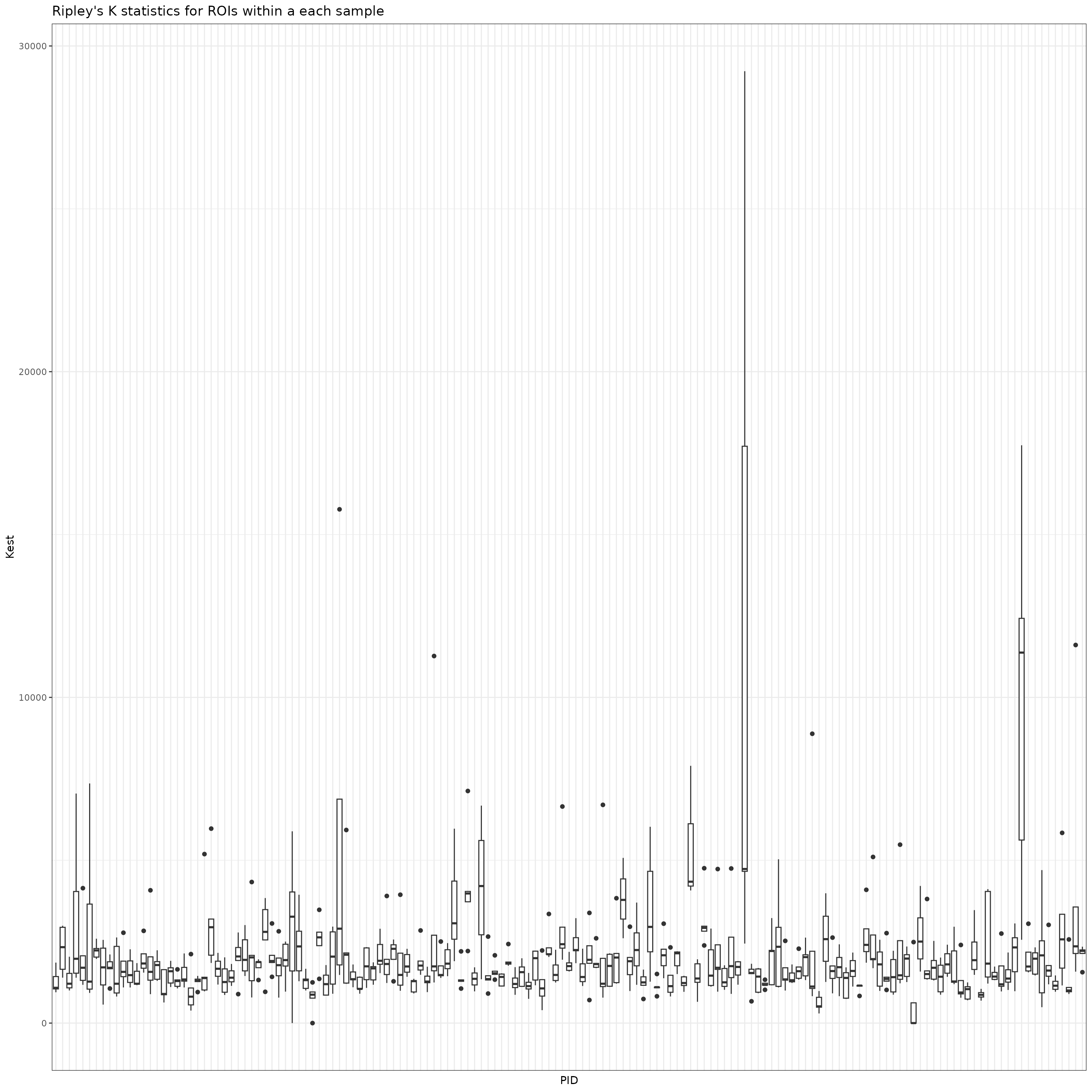
We now compute the weighted averages given above as well as a standard arithmetic mean as a comparison. Below, we visualize the spread of the various spatial aggregation methods within each sample.
# Compute averages
results_mean <- results %>%
    dplyr::group_by(PID) %>%
    dplyr::summarise_at(dplyr::vars(spatial),
                        list(~mean(.x),
                             ~landau.avg(K.vec = .x, area.vec = area, n.vec = npoints),
                             ~diggle.avg(K.vec = .x, n.vec = npoints),
                             ~baddeley.avg(K.vec = .x, n.vec = npoints)))

# Plot the averages
results_mean %>%
  tidyr::pivot_longer(2:5, names_to = "mean", values_to = "value") %>%
  dplyr::mutate(mean = recode(mean,
                              "mean" = "Arithmetic Mean",
                              "landau.avg" = "Landau Mean",
                              "diggle.avg" = "Diggle Mean",
                              "baddeley.avg" = "Baddeley Mean")) %>%
  ggplot(aes(x = PID, y = value, group = mean, color = mean)) +
  geom_point() +
  theme_bw() +
  theme(axis.text.x = element_blank(),
        axis.ticks.x = element_blank()) +
  ylab("Average Kest") +
  ggtitle("Averaged Ripley's K within each sample") +
  scale_color_discrete(name = "Aggregation Method")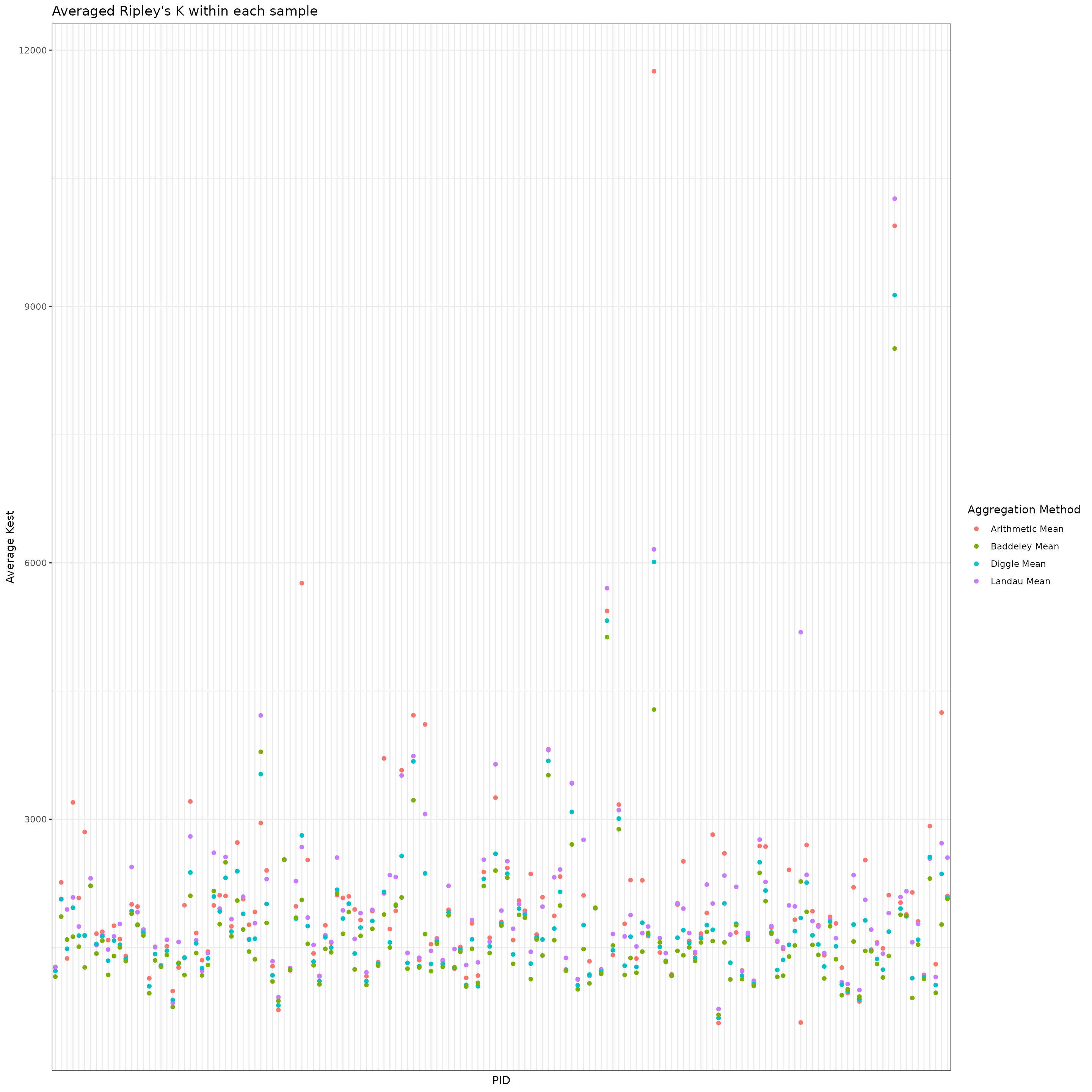
We now have a data.frame with a column corresponding to each average. Let’s add in the MHCII-high status variable so we can do association testing. We would like to test if the spatial colocalization of tumor and CD4+ T cells is associated with MHCII-high status, adjusting for patient age. We will compare the significance of this association across the four spatial aggregation methods.
# First, check the ordering matches
all(unique(lung_df_tumor$PID) == results_mean$PID) # TRUE!
#> [1] TRUE

# Add in MHCII-high status and age
results_mean <- cbind.data.frame(
  results_mean,
  lung_df_tumor %>%
    dplyr::select(PID, mhcII_high, age_at_diagnosis) %>%
    dplyr::distinct() %>%
    dplyr::select(mhcII_high, age_at_diagnosis)
)

# Test for an association between CD4 T cell spatial distributions and MHCII-high status
mean.glm <- glm(mhcII_high ~ mean + age_at_diagnosis, data = results_mean, family = binomial())
diggle.glm <- glm(mhcII_high ~ diggle.avg + age_at_diagnosis, data = results_mean, family = binomial())
baddeley.glm <- glm(mhcII_high ~ baddeley.avg + age_at_diagnosis, data = results_mean, family = binomial())
landau.glm <- glm(mhcII_high ~ landau.avg + age_at_diagnosis, data = results_mean, family = binomial())

# Save the p-values in a table and display
cd4.tumor.pvals <- data.frame(
  Method = c("Mean", "Diggle", "Baddeley", "Landau"),
  P.Value = c(summary(mean.glm)$coef[2,4], summary(diggle.glm)$coef[2,4],
              summary(baddeley.glm)$coef[2,4], summary(landau.glm)$coef[2,4])
)

# Show the results
cd4.tumor.pvals
#>     Method    P.Value
#> 1     Mean 0.03579355
#> 2   Diggle 0.02336449
#> 3 Baddeley 0.02962022
#> 4   Landau 0.06036164
Using the mean, Diggle, and Baddeley approaches, we found a significant association between the spatial colocalization of CD4+ T cells and tumors with MHCII-high status. We did not find a significant association using the Landau mean, however. The Landau mean accounts for variation in the intensity across ROIs which, in this case, may not have been informative for understanding the relationship between cell colocalizations and outcomes.
Ensemble Approaches
We now illustrate using ensemble testing to test the same hypothesis. These ensemble approaches consider multiple random weights used to construct the aggregations of the spatial summary statistics. For each set of random weights, we test for an association between the weighted aggregation and outcome. We repeat this for many random weights and combine the resulting p-values using a p-value combination method. For this purpose, we use the Cauchy combination test (Liu and Xie (2020)).
The motivation behind these ensemble approaches is that the best set of weights (the weights that will yield the highest power) is generally unknown at the outset. For this reason, considering many different possible weights may gain us more power because we may capture the true relationship between the aggregated spatial summary statistics and sample-level outcome.
spagg contains implementations for two different
approaches which are introduced in the Getting Started
vignette:
Standard ensemble testing
Combination testing
We now run each of these approaches to testing using the
results data.frame we constructed above.
# Add the outcome back into the data
results <- left_join(results,
                     lung_df_tumor %>% dplyr::select(id, PID, mhcII_high, age_at_diagnosis) %>% distinct(),
                     by = c("id", "PID"))

# Run each ensemble test
ensemble.res <- ensemble.avg(data = results,
                             group = "PID",
                             adjustments = "age_at_diagnosis",
                             outcome = "mhcII_high",
                             model = "logistic")

combo.res <- combo.weight.avg(data = results,
                              group = "PID",
                              adjustments = "age_at_diagnosis",
                              outcome = "mhcII_high",
                              model = "logistic")

# Add the results to the results data.frame
cd4.tumor.pvals <- rbind.data.frame(
  cd4.tumor.pvals,
  data.frame(
    Method = c("Ensemble", "Combo"),
    P.Value = c(ensemble.res$pval, combo.res$pval)
  )
)

# Display
cd4.tumor.pvals
#>     Method    P.Value
#> 1     Mean 0.03579355
#> 2   Diggle 0.02336449
#> 3 Baddeley 0.02962022
#> 4   Landau 0.06036164
#> 5 Ensemble 0.02574108
#> 6    Combo 0.02081173
Across all approaches, we found that there was a significant association between spatial colocalization of CD4+ T cells and tumor cells with MHCII-high status.