Application of TopKAT to a Study of Triple Negative Breast Cancer
tnbc_application.RmdPackage and Data Import
This vignette demonstrates the application of TopKAT to a study in triple negative breast cancer (TNBC) using MIBI-TOF to probe the tumor microenvironment in breast cancer biopsies. The data was originally published in Keren et al. (2018).
Keren et al. observed that tumor biopsies could be categorized based
on the degree of mixing between immune cells and tumor cells. In some
biopsies, immune and tumor cells colocalized and interspersed together
throughout the tumor. These biopsies were referred to as
mixed" biopsies. In others, immune cells and tumor cells segregated into different regions, forming connected components and loops around each other. These biopsies were calledcompartmentalized.”
Finally, some biopsies contained very few immune cells altogether and
were referred to as a ``cold” biopsies. The apparent differences in
spatial patterns among immune cells across these biopsies motivated this
as an application of TopKAT, which we illustrate here.
The dataset, tnbc is lazily loaded with the import of
the TopKAT package. We start by importing packages we will
need for our analysis.
# Packages
library(TopKAT)
library(dplyr)
library(ACAT)
library(ggplot2)
library(tidyr)
library(gtools)
library(MiRKAT)
library(TDAstats)
library(viridis)
library(patchwork)

# Load in the data
data(tnbc)
We first save perform some basics with the data. We label the cell types identified in the data, including non-immune cells (tumor cells, epithelial cells, mesenchymal cells, and endothelial cells) and several immune cell types, including Tregs, CD4 T cells, CD8 T cells, CD3 T cells, NK cells, B cells, neutrophils, macrophages, dendritic cells, DC/monocytes, monocytes/neutrophils, and other unidentified cell types. We have filtered the dataset already to include just immune and keratin-positive tumor cells. The documentation for the cell types is published online alongside the original publication.
We also save the number of biopsies in this dataset, from 38 different patients.
# Label the cell types
tnbc$immuneGroup <- factor(tnbc$immuneGroup)
levels(tnbc$immuneGroup) <- c("Non-Immune", "Treg", "CD4 T", "CD8 T", "CD3 T", "NK",
                              "B cell", "Neutrophil", "Macrophage", "Dendritic",
                              "DC/Mono", "Mono/Neu", "Other")

# Rename and save the patient IDs
PIDs <- as.numeric(unique(tnbc$SampleID))

# Save the number of patients
n <- length(PIDs)
The biopsy categories (mixed, compartmentalized, cold) are given in
the column tnbc$Class which has three levels, 0, 1, and 2.
The coding is as follows:
- 0 = mixed
- 1 = compartmentalized
- 2 = cold
Below, we demonstrate several images from the dataset to demonstrate the different patterns among immune cells and tumor cells. The classification of the biopsies is given in the figure titles. The figures illustrate that mixed samples show a scatter of immune and tumor cells throughout the tumor microenvironment, whereas compartmentalized samples show distinct clusters of immune cells separate from tumor cells.
p1_ti <- tnbc %>%
  filter(SampleID == 1) %>%
  mutate(Group = factor(Group)) %>%
  ggplot(aes(x = x, y = y, fill = Group)) +
  geom_point(color = "black", pch = 21) +
  theme_bw() +
  viridis::scale_fill_viridis(discrete = TRUE, begin = 0.35, end = 0.75,
                             labels = c("Immune", "Tumor"),
                             name = "Cell Type") +
  ggtitle("Example Image from Patient 1 (Mixed)")

p2_ti <- tnbc %>%
  filter(SampleID == 2) %>%
  mutate(Group = factor(Group)) %>%
  ggplot(aes(x = x, y = y, fill = Group)) +
  geom_point(color = "black", pch = 21) +
  theme_bw() +
  viridis::scale_fill_viridis(discrete = TRUE, begin = 0.35, end = 0.75,
                             labels = c("Immune", "Tumor"),
                             name = "Cell Type") +
  ggtitle("Example Image from Patient 2 (Mixed)")

p3_ti <- tnbc %>%
  filter(SampleID == 3) %>%
  mutate(Group = factor(Group)) %>%
  ggplot(aes(x = x, y = y, fill = Group)) +
  geom_point(color = "black", pch = 21) +
  theme_bw() +
  viridis::scale_fill_viridis(discrete = TRUE, begin = 0.35, end = 0.75,
                             labels = c("Immune", "Tumor"),
                             name = "Cell Type") +
  ggtitle("Example Image from Patient 3 (Compartmentalized)")

p4_ti <- tnbc %>%
  filter(SampleID == 4) %>%
  mutate(Group = factor(Group)) %>%
  ggplot(aes(x = x, y = y, fill = Group)) +
  geom_point(color = "black", pch = 21) +
  theme_bw() +
  viridis::scale_fill_viridis(discrete = TRUE, begin = 0.35, end = 0.75,
                             labels = c("Immune", "Tumor"),
                             name = "Cell Type") +
  ggtitle("Example Image from Patient 4 (Compartmentalized)")

# Plot
p1_ti + p2_ti +
  p3_ti + p4_ti +
  plot_layout(ncol = 2, nrow = 2)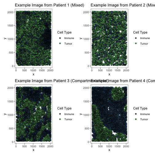
The goals of this analysis are two-fold. The first goal is to relate the topological structures among immune cells to overall patient survival. The second is to describe the distinctions among mixed, compartmentalized, and cold samples topologically. For both goals, we focus on capturing the topological structures created by just the immune cells.
To address both goals, we are going to be applying TopKAT to just the immune cells. Below, we visualize the same figures above with just the immune cells shown.
p1_i <- tnbc %>%
  filter(SampleID == 1) %>%
  filter(Group == 2) %>%
  mutate(Group = factor(Group)) %>%
  ggplot(aes(x = x, y = y, fill = Group)) +
  geom_point(color = "black", pch = 21) +
  theme_bw() +
  viridis::scale_fill_viridis(discrete = TRUE, begin = 0.35, end = 0.75,
                             labels = c("Immune"),
                             name = "Cell Type") +
  ggtitle("Example Image from Patient 1 (Mixed)")

p2_i <- tnbc %>%
  filter(SampleID == 2) %>%
  filter(Group == 2) %>%
  mutate(Group = factor(Group)) %>%
  ggplot(aes(x = x, y = y, fill = Group)) +
  geom_point(color = "black", pch = 21) +
  theme_bw() +
  viridis::scale_fill_viridis(discrete = TRUE, begin = 0.35, end = 0.75,
                             labels = c("Immune"),
                             name = "Cell Type") +
  ggtitle("Example Image from Patient 2 (Mixed)")

p3_i <- tnbc %>%
  filter(SampleID == 3) %>%
  filter(Group == 2) %>%
  mutate(Group = factor(Group)) %>%
  ggplot(aes(x = x, y = y, fill = Group)) +
  geom_point(color = "black", pch = 21) +
  theme_bw() +
  viridis::scale_fill_viridis(discrete = TRUE, begin = 0.35, end = 0.75,
                             labels = c("Immune"),
                             name = "Cell Type") +
  ggtitle("Example Image from Patient 3 (Compartmentalized)")

p4_i <- tnbc %>%
  filter(SampleID == 4) %>%
  filter(Group == 2) %>%
  mutate(Group = factor(Group)) %>%
  ggplot(aes(x = x, y = y, fill = Group)) +
  geom_point(color = "black", pch = 21) +
  theme_bw() +
  viridis::scale_fill_viridis(discrete = TRUE, begin = 0.35, end = 0.75,
                             labels = c("Immune"),
                             name = "Cell Type") +
  ggtitle("Example Image from Patient 4 (Compartmentalized)")

p1_i + p2_i +
  p3_i + p4_i +
  plot_layout(ncol = 2, nrow = 2)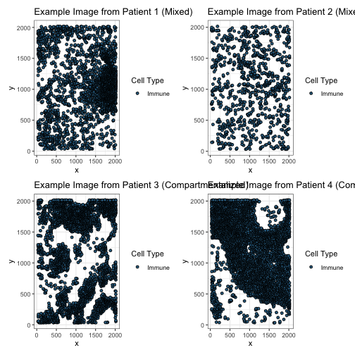
Applying TopKAT
The first step in applying TopKAT is to construct a filtration. The process of filtration creates a series of nested graphs where each cell is a node and edges are drawn between cells if they are no more than some distance apart. The goal of applying a filtration is to capture the size (or ``lifespan”) of homologies created among the, in our case, immune cells. Homologies are the topological structures (connected components and loops), which we wish to capture.
We first subset the data to just the immune cells (denoted by ``Group == 2”). We then construct a Rips filtration for each image on the basis of just the immune cells. The topological structures detected throughout filtration are summarized in a summary statistic called a persistence diagram, which are visualized below.
# Save just the immune cells
tnbc.immune <- tnbc %>% filter(Group == 2)
tnbc.immune$immuneGroup <- droplevels(tnbc.immune$immuneGroup)

# Create a list to store the PDs
PD.list <- lapply(1:n, function(i) list())

# Iterate through the IDs and generate a Rips complex for the immune cells
for (i in PIDs) {

  # Print progress
  print(paste0(which(PIDs %in% i), "/", length(PIDs)))

  # Subset the data to just this PID
  data.i <- tnbc.immune %>%
    filter(SampleID == i) %>%
    dplyr::select(x,y)

  # Construct a Rips filtration using TDAstats
  rips.i <- TDAstats::calculate_homology(data.i, dim = 1, threshold = 2048)

  # Save the results
  PD.list[[which(PIDs %in% i)]] <- rips.i
}
#> [1] "1/38"
#> [1] "2/38"
#> [1] "3/38"
#> [1] "4/38"
#> [1] "5/38"
#> [1] "6/38"
#> [1] "7/38"
#> [1] "8/38"
#> [1] "9/38"
#> [1] "10/38"
#> [1] "11/38"
#> [1] "12/38"
#> [1] "13/38"
#> [1] "14/38"
#> [1] "15/38"
#> [1] "16/38"
#> [1] "17/38"
#> [1] "18/38"
#> [1] "19/38"
#> [1] "20/38"
#> [1] "21/38"
#> [1] "22/38"
#> [1] "23/38"
#> [1] "24/38"
#> [1] "25/38"
#> [1] "26/38"
#> [1] "27/38"
#> [1] "28/38"
#> [1] "29/38"
#> [1] "30/38"
#> [1] "31/38"
#> [1] "32/38"
#> [1] "33/38"
#> [1] "34/38"
#> [1] "35/38"
#> [1] "36/38"
#> [1] "37/38"
#> [1] "38/38"

# Visualize a few examples
pd1 <- plot_persistence(PD.list[[1]], title = "Sample 1 (Mixed)", dims = c(300, 300))
pd2 <- plot_persistence(PD.list[[2]], title = "Sample 2 (Mixed)", dims = c(300, 300))
pd3 <- plot_persistence(PD.list[[1]], title = "Sample 3 \n (Compartmentalized)", dims = c(300, 300))
pd4 <- plot_persistence(PD.list[[2]], title = "Sample 4 \n (Compartmentalized)", dims = c(300, 300))

pd1 + pd2 +
  pd3 + pd4 +
  plot_layout(ncol = 2, nrow = 2)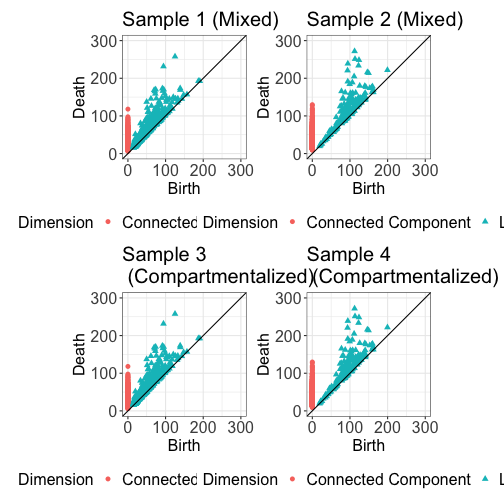
knitr::include_graphics("vignettes/figures/immune_cell_filtration_1.png", error = FALSE)
After we have calculated a persistence diagram for each image, we then can associate these persistence diagrams with an outcome. To do this, we use a kernel machine regression framework. For this, we need to construct a kernel matrix which quantifies the similarities among pairs of persistence diagrams. To obtain a kernel matrix, we first start by calculating a pairwise dissimilarity matrix. The process then is:
- Calculate pairwise dissimilarity matrix between persistence diagrams
- Convert the pairwise dissimilarity matrix to a pairwise kernel matrix to quantify similarity (rather than dissimilarity)
- Input kernel matrix in a kernel machine regression framework with an outcome.
The construction of the dissimilarity and kernel matrices occurs separately for both connected components and loops. We first start by generating pairs of sample IDs to iterate through. Then we initialize our pairwise distance matrices. Then we iterate through all the pairs of persistence diagrams and calculate the distance between them.
# Create all pairs of samples
pairs <- gtools::combinations(n = n, r = 2, v = sort(PIDs), repeats.allowed = FALSE)

# Initialize a distance matrix (comparing the matrices based on distance)
dist.mat.deg0 <- dist.mat.deg1 <- matrix(0, nrow = n, ncol = n)

# Add names
rownames(dist.mat.deg0) <- colnames(dist.mat.deg0) <-
  rownames(dist.mat.deg1) <- colnames(dist.mat.deg1) <-
  PIDs

# Iterate through pairs and calculate distance
for (i in 1:nrow(pairs)) {

  # Print progress
  print(paste0(i, "/", nrow(pairs)))

  # Save the current pair
  ids <- pairs[i,]
  id.1 <- ids[1]
  id.2 <- ids[2]

  # Load in the diagrams
  rips.1 <- PD.list[[which(PIDs %in% id.1)]]
  rips.2 <- PD.list[[which(PIDs %in% id.2)]]

  # Calculate distance
  dist.i <- phom.dist(rips.1, rips.2)

  # Save the results
  row.ind <- which(rownames(dist.mat.deg0) == id.1)
  col.ind <- which(rownames(dist.mat.deg0) == id.2)

  dist.mat.deg0[row.ind, col.ind] <- dist.i[1]
  dist.mat.deg1[row.ind, col.ind] <- dist.i[2]
}
#> [1] "1/703"
#> [1] "2/703"
#> [1] "3/703"
#> [1] "4/703"
#> [1] "5/703"
#> [1] "6/703"
#> [1] "7/703"
#> [1] "8/703"
#> [1] "9/703"
#> [1] "10/703"
#> [1] "11/703"
#> [1] "12/703"
#> [1] "13/703"
#> [1] "14/703"
#> [1] "15/703"
#> [1] "16/703"
#> [1] "17/703"
#> [1] "18/703"
#> [1] "19/703"
#> [1] "20/703"
#> [1] "21/703"
#> [1] "22/703"
#> [1] "23/703"
#> [1] "24/703"
#> [1] "25/703"
#> [1] "26/703"
#> [1] "27/703"
#> [1] "28/703"
#> [1] "29/703"
#> [1] "30/703"
#> [1] "31/703"
#> [1] "32/703"
#> [1] "33/703"
#> [1] "34/703"
#> [1] "35/703"
#> [1] "36/703"
#> [1] "37/703"
#> [1] "38/703"
#> [1] "39/703"
#> [1] "40/703"
#> [1] "41/703"
#> [1] "42/703"
#> [1] "43/703"
#> [1] "44/703"
#> [1] "45/703"
#> [1] "46/703"
#> [1] "47/703"
#> [1] "48/703"
#> [1] "49/703"
#> [1] "50/703"
#> [1] "51/703"
#> [1] "52/703"
#> [1] "53/703"
#> [1] "54/703"
#> [1] "55/703"
#> [1] "56/703"
#> [1] "57/703"
#> [1] "58/703"
#> [1] "59/703"
#> [1] "60/703"
#> [1] "61/703"
#> [1] "62/703"
#> [1] "63/703"
#> [1] "64/703"
#> [1] "65/703"
#> [1] "66/703"
#> [1] "67/703"
#> [1] "68/703"
#> [1] "69/703"
#> [1] "70/703"
#> [1] "71/703"
#> [1] "72/703"
#> [1] "73/703"
#> [1] "74/703"
#> [1] "75/703"
#> [1] "76/703"
#> [1] "77/703"
#> [1] "78/703"
#> [1] "79/703"
#> [1] "80/703"
#> [1] "81/703"
#> [1] "82/703"
#> [1] "83/703"
#> [1] "84/703"
#> [1] "85/703"
#> [1] "86/703"
#> [1] "87/703"
#> [1] "88/703"
#> [1] "89/703"
#> [1] "90/703"
#> [1] "91/703"
#> [1] "92/703"
#> [1] "93/703"
#> [1] "94/703"
#> [1] "95/703"
#> [1] "96/703"
#> [1] "97/703"
#> [1] "98/703"
#> [1] "99/703"
#> [1] "100/703"
#> [1] "101/703"
#> [1] "102/703"
#> [1] "103/703"
#> [1] "104/703"
#> [1] "105/703"
#> [1] "106/703"
#> [1] "107/703"
#> [1] "108/703"
#> [1] "109/703"
#> [1] "110/703"
#> [1] "111/703"
#> [1] "112/703"
#> [1] "113/703"
#> [1] "114/703"
#> [1] "115/703"
#> [1] "116/703"
#> [1] "117/703"
#> [1] "118/703"
#> [1] "119/703"
#> [1] "120/703"
#> [1] "121/703"
#> [1] "122/703"
#> [1] "123/703"
#> [1] "124/703"
#> [1] "125/703"
#> [1] "126/703"
#> [1] "127/703"
#> [1] "128/703"
#> [1] "129/703"
#> [1] "130/703"
#> [1] "131/703"
#> [1] "132/703"
#> [1] "133/703"
#> [1] "134/703"
#> [1] "135/703"
#> [1] "136/703"
#> [1] "137/703"
#> [1] "138/703"
#> [1] "139/703"
#> [1] "140/703"
#> [1] "141/703"
#> [1] "142/703"
#> [1] "143/703"
#> [1] "144/703"
#> [1] "145/703"
#> [1] "146/703"
#> [1] "147/703"
#> [1] "148/703"
#> [1] "149/703"
#> [1] "150/703"
#> [1] "151/703"
#> [1] "152/703"
#> [1] "153/703"
#> [1] "154/703"
#> [1] "155/703"
#> [1] "156/703"
#> [1] "157/703"
#> [1] "158/703"
#> [1] "159/703"
#> [1] "160/703"
#> [1] "161/703"
#> [1] "162/703"
#> [1] "163/703"
#> [1] "164/703"
#> [1] "165/703"
#> [1] "166/703"
#> [1] "167/703"
#> [1] "168/703"
#> [1] "169/703"
#> [1] "170/703"
#> [1] "171/703"
#> [1] "172/703"
#> [1] "173/703"
#> [1] "174/703"
#> [1] "175/703"
#> [1] "176/703"
#> [1] "177/703"
#> [1] "178/703"
#> [1] "179/703"
#> [1] "180/703"
#> [1] "181/703"
#> [1] "182/703"
#> [1] "183/703"
#> [1] "184/703"
#> [1] "185/703"
#> [1] "186/703"
#> [1] "187/703"
#> [1] "188/703"
#> [1] "189/703"
#> [1] "190/703"
#> [1] "191/703"
#> [1] "192/703"
#> [1] "193/703"
#> [1] "194/703"
#> [1] "195/703"
#> [1] "196/703"
#> [1] "197/703"
#> [1] "198/703"
#> [1] "199/703"
#> [1] "200/703"
#> [1] "201/703"
#> [1] "202/703"
#> [1] "203/703"
#> [1] "204/703"
#> [1] "205/703"
#> [1] "206/703"
#> [1] "207/703"
#> [1] "208/703"
#> [1] "209/703"
#> [1] "210/703"
#> [1] "211/703"
#> [1] "212/703"
#> [1] "213/703"
#> [1] "214/703"
#> [1] "215/703"
#> [1] "216/703"
#> [1] "217/703"
#> [1] "218/703"
#> [1] "219/703"
#> [1] "220/703"
#> [1] "221/703"
#> [1] "222/703"
#> [1] "223/703"
#> [1] "224/703"
#> [1] "225/703"
#> [1] "226/703"
#> [1] "227/703"
#> [1] "228/703"
#> [1] "229/703"
#> [1] "230/703"
#> [1] "231/703"
#> [1] "232/703"
#> [1] "233/703"
#> [1] "234/703"
#> [1] "235/703"
#> [1] "236/703"
#> [1] "237/703"
#> [1] "238/703"
#> [1] "239/703"
#> [1] "240/703"
#> [1] "241/703"
#> [1] "242/703"
#> [1] "243/703"
#> [1] "244/703"
#> [1] "245/703"
#> [1] "246/703"
#> [1] "247/703"
#> [1] "248/703"
#> [1] "249/703"
#> [1] "250/703"
#> [1] "251/703"
#> [1] "252/703"
#> [1] "253/703"
#> [1] "254/703"
#> [1] "255/703"
#> [1] "256/703"
#> [1] "257/703"
#> [1] "258/703"
#> [1] "259/703"
#> [1] "260/703"
#> [1] "261/703"
#> [1] "262/703"
#> [1] "263/703"
#> [1] "264/703"
#> [1] "265/703"
#> [1] "266/703"
#> [1] "267/703"
#> [1] "268/703"
#> [1] "269/703"
#> [1] "270/703"
#> [1] "271/703"
#> [1] "272/703"
#> [1] "273/703"
#> [1] "274/703"
#> [1] "275/703"
#> [1] "276/703"
#> [1] "277/703"
#> [1] "278/703"
#> [1] "279/703"
#> [1] "280/703"
#> [1] "281/703"
#> [1] "282/703"
#> [1] "283/703"
#> [1] "284/703"
#> [1] "285/703"
#> [1] "286/703"
#> [1] "287/703"
#> [1] "288/703"
#> [1] "289/703"
#> [1] "290/703"
#> [1] "291/703"
#> [1] "292/703"
#> [1] "293/703"
#> [1] "294/703"
#> [1] "295/703"
#> [1] "296/703"
#> [1] "297/703"
#> [1] "298/703"
#> [1] "299/703"
#> [1] "300/703"
#> [1] "301/703"
#> [1] "302/703"
#> [1] "303/703"
#> [1] "304/703"
#> [1] "305/703"
#> [1] "306/703"
#> [1] "307/703"
#> [1] "308/703"
#> [1] "309/703"
#> [1] "310/703"
#> [1] "311/703"
#> [1] "312/703"
#> [1] "313/703"
#> [1] "314/703"
#> [1] "315/703"
#> [1] "316/703"
#> [1] "317/703"
#> [1] "318/703"
#> [1] "319/703"
#> [1] "320/703"
#> [1] "321/703"
#> [1] "322/703"
#> [1] "323/703"
#> [1] "324/703"
#> [1] "325/703"
#> [1] "326/703"
#> [1] "327/703"
#> [1] "328/703"
#> [1] "329/703"
#> [1] "330/703"
#> [1] "331/703"
#> [1] "332/703"
#> [1] "333/703"
#> [1] "334/703"
#> [1] "335/703"
#> [1] "336/703"
#> [1] "337/703"
#> [1] "338/703"
#> [1] "339/703"
#> [1] "340/703"
#> [1] "341/703"
#> [1] "342/703"
#> [1] "343/703"
#> [1] "344/703"
#> [1] "345/703"
#> [1] "346/703"
#> [1] "347/703"
#> [1] "348/703"
#> [1] "349/703"
#> [1] "350/703"
#> [1] "351/703"
#> [1] "352/703"
#> [1] "353/703"
#> [1] "354/703"
#> [1] "355/703"
#> [1] "356/703"
#> [1] "357/703"
#> [1] "358/703"
#> [1] "359/703"
#> [1] "360/703"
#> [1] "361/703"
#> [1] "362/703"
#> [1] "363/703"
#> [1] "364/703"
#> [1] "365/703"
#> [1] "366/703"
#> [1] "367/703"
#> [1] "368/703"
#> [1] "369/703"
#> [1] "370/703"
#> [1] "371/703"
#> [1] "372/703"
#> [1] "373/703"
#> [1] "374/703"
#> [1] "375/703"
#> [1] "376/703"
#> [1] "377/703"
#> [1] "378/703"
#> [1] "379/703"
#> [1] "380/703"
#> [1] "381/703"
#> [1] "382/703"
#> [1] "383/703"
#> [1] "384/703"
#> [1] "385/703"
#> [1] "386/703"
#> [1] "387/703"
#> [1] "388/703"
#> [1] "389/703"
#> [1] "390/703"
#> [1] "391/703"
#> [1] "392/703"
#> [1] "393/703"
#> [1] "394/703"
#> [1] "395/703"
#> [1] "396/703"
#> [1] "397/703"
#> [1] "398/703"
#> [1] "399/703"
#> [1] "400/703"
#> [1] "401/703"
#> [1] "402/703"
#> [1] "403/703"
#> [1] "404/703"
#> [1] "405/703"
#> [1] "406/703"
#> [1] "407/703"
#> [1] "408/703"
#> [1] "409/703"
#> [1] "410/703"
#> [1] "411/703"
#> [1] "412/703"
#> [1] "413/703"
#> [1] "414/703"
#> [1] "415/703"
#> [1] "416/703"
#> [1] "417/703"
#> [1] "418/703"
#> [1] "419/703"
#> [1] "420/703"
#> [1] "421/703"
#> [1] "422/703"
#> [1] "423/703"
#> [1] "424/703"
#> [1] "425/703"
#> [1] "426/703"
#> [1] "427/703"
#> [1] "428/703"
#> [1] "429/703"
#> [1] "430/703"
#> [1] "431/703"
#> [1] "432/703"
#> [1] "433/703"
#> [1] "434/703"
#> [1] "435/703"
#> [1] "436/703"
#> [1] "437/703"
#> [1] "438/703"
#> [1] "439/703"
#> [1] "440/703"
#> [1] "441/703"
#> [1] "442/703"
#> [1] "443/703"
#> [1] "444/703"
#> [1] "445/703"
#> [1] "446/703"
#> [1] "447/703"
#> [1] "448/703"
#> [1] "449/703"
#> [1] "450/703"
#> [1] "451/703"
#> [1] "452/703"
#> [1] "453/703"
#> [1] "454/703"
#> [1] "455/703"
#> [1] "456/703"
#> [1] "457/703"
#> [1] "458/703"
#> [1] "459/703"
#> [1] "460/703"
#> [1] "461/703"
#> [1] "462/703"
#> [1] "463/703"
#> [1] "464/703"
#> [1] "465/703"
#> [1] "466/703"
#> [1] "467/703"
#> [1] "468/703"
#> [1] "469/703"
#> [1] "470/703"
#> [1] "471/703"
#> [1] "472/703"
#> [1] "473/703"
#> [1] "474/703"
#> [1] "475/703"
#> [1] "476/703"
#> [1] "477/703"
#> [1] "478/703"
#> [1] "479/703"
#> [1] "480/703"
#> [1] "481/703"
#> [1] "482/703"
#> [1] "483/703"
#> [1] "484/703"
#> [1] "485/703"
#> [1] "486/703"
#> [1] "487/703"
#> [1] "488/703"
#> [1] "489/703"
#> [1] "490/703"
#> [1] "491/703"
#> [1] "492/703"
#> [1] "493/703"
#> [1] "494/703"
#> [1] "495/703"
#> [1] "496/703"
#> [1] "497/703"
#> [1] "498/703"
#> [1] "499/703"
#> [1] "500/703"
#> [1] "501/703"
#> [1] "502/703"
#> [1] "503/703"
#> [1] "504/703"
#> [1] "505/703"
#> [1] "506/703"
#> [1] "507/703"
#> [1] "508/703"
#> [1] "509/703"
#> [1] "510/703"
#> [1] "511/703"
#> [1] "512/703"
#> [1] "513/703"
#> [1] "514/703"
#> [1] "515/703"
#> [1] "516/703"
#> [1] "517/703"
#> [1] "518/703"
#> [1] "519/703"
#> [1] "520/703"
#> [1] "521/703"
#> [1] "522/703"
#> [1] "523/703"
#> [1] "524/703"
#> [1] "525/703"
#> [1] "526/703"
#> [1] "527/703"
#> [1] "528/703"
#> [1] "529/703"
#> [1] "530/703"
#> [1] "531/703"
#> [1] "532/703"
#> [1] "533/703"
#> [1] "534/703"
#> [1] "535/703"
#> [1] "536/703"
#> [1] "537/703"
#> [1] "538/703"
#> [1] "539/703"
#> [1] "540/703"
#> [1] "541/703"
#> [1] "542/703"
#> [1] "543/703"
#> [1] "544/703"
#> [1] "545/703"
#> [1] "546/703"
#> [1] "547/703"
#> [1] "548/703"
#> [1] "549/703"
#> [1] "550/703"
#> [1] "551/703"
#> [1] "552/703"
#> [1] "553/703"
#> [1] "554/703"
#> [1] "555/703"
#> [1] "556/703"
#> [1] "557/703"
#> [1] "558/703"
#> [1] "559/703"
#> [1] "560/703"
#> [1] "561/703"
#> [1] "562/703"
#> [1] "563/703"
#> [1] "564/703"
#> [1] "565/703"
#> [1] "566/703"
#> [1] "567/703"
#> [1] "568/703"
#> [1] "569/703"
#> [1] "570/703"
#> [1] "571/703"
#> [1] "572/703"
#> [1] "573/703"
#> [1] "574/703"
#> [1] "575/703"
#> [1] "576/703"
#> [1] "577/703"
#> [1] "578/703"
#> [1] "579/703"
#> [1] "580/703"
#> [1] "581/703"
#> [1] "582/703"
#> [1] "583/703"
#> [1] "584/703"
#> [1] "585/703"
#> [1] "586/703"
#> [1] "587/703"
#> [1] "588/703"
#> [1] "589/703"
#> [1] "590/703"
#> [1] "591/703"
#> [1] "592/703"
#> [1] "593/703"
#> [1] "594/703"
#> [1] "595/703"
#> [1] "596/703"
#> [1] "597/703"
#> [1] "598/703"
#> [1] "599/703"
#> [1] "600/703"
#> [1] "601/703"
#> [1] "602/703"
#> [1] "603/703"
#> [1] "604/703"
#> [1] "605/703"
#> [1] "606/703"
#> [1] "607/703"
#> [1] "608/703"
#> [1] "609/703"
#> [1] "610/703"
#> [1] "611/703"
#> [1] "612/703"
#> [1] "613/703"
#> [1] "614/703"
#> [1] "615/703"
#> [1] "616/703"
#> [1] "617/703"
#> [1] "618/703"
#> [1] "619/703"
#> [1] "620/703"
#> [1] "621/703"
#> [1] "622/703"
#> [1] "623/703"
#> [1] "624/703"
#> [1] "625/703"
#> [1] "626/703"
#> [1] "627/703"
#> [1] "628/703"
#> [1] "629/703"
#> [1] "630/703"
#> [1] "631/703"
#> [1] "632/703"
#> [1] "633/703"
#> [1] "634/703"
#> [1] "635/703"
#> [1] "636/703"
#> [1] "637/703"
#> [1] "638/703"
#> [1] "639/703"
#> [1] "640/703"
#> [1] "641/703"
#> [1] "642/703"
#> [1] "643/703"
#> [1] "644/703"
#> [1] "645/703"
#> [1] "646/703"
#> [1] "647/703"
#> [1] "648/703"
#> [1] "649/703"
#> [1] "650/703"
#> [1] "651/703"
#> [1] "652/703"
#> [1] "653/703"
#> [1] "654/703"
#> [1] "655/703"
#> [1] "656/703"
#> [1] "657/703"
#> [1] "658/703"
#> [1] "659/703"
#> [1] "660/703"
#> [1] "661/703"
#> [1] "662/703"
#> [1] "663/703"
#> [1] "664/703"
#> [1] "665/703"
#> [1] "666/703"
#> [1] "667/703"
#> [1] "668/703"
#> [1] "669/703"
#> [1] "670/703"
#> [1] "671/703"
#> [1] "672/703"
#> [1] "673/703"
#> [1] "674/703"
#> [1] "675/703"
#> [1] "676/703"
#> [1] "677/703"
#> [1] "678/703"
#> [1] "679/703"
#> [1] "680/703"
#> [1] "681/703"
#> [1] "682/703"
#> [1] "683/703"
#> [1] "684/703"
#> [1] "685/703"
#> [1] "686/703"
#> [1] "687/703"
#> [1] "688/703"
#> [1] "689/703"
#> [1] "690/703"
#> [1] "691/703"
#> [1] "692/703"
#> [1] "693/703"
#> [1] "694/703"
#> [1] "695/703"
#> [1] "696/703"
#> [1] "697/703"
#> [1] "698/703"
#> [1] "699/703"
#> [1] "700/703"
#> [1] "701/703"
#> [1] "702/703"
#> [1] "703/703"
Now that we have our distance matrices prepared, we can convert them
to kernel matrices and input them in our kernel machine regression
framework. We start by filling in the lower triangular portion of the
distance matrix (since we only filled in the upper half above). We then
convert it to a kernel matrix using a Gower centered kernel with the
function MiRKAT::D2K function. Since we have two kernel
matrices, we consider a sequence of linear combinations of the two in
our test. We start by testing for an association with just the kernel
matrix based on connected components
(
in the code), based on a 50-50 even contribution from both kernel
matrices
(),
and just the kernel matrix based on loops
().
For our first analytical goal, we test for an association with overall survival. Below, we demonstrate how to extract the survival times, censoring indicator, and age of each patient, which we adjust for in our test.
The resulting kernel association testing p-value is printed below. We observed a significant association in the topological structures among immune cells and overall survival.
# Convert the distance matrices to symmetric matrices
dist.mat.deg0 <- dist.mat.deg0 + t(dist.mat.deg0)
dist.mat.deg1 <- dist.mat.deg1 + t(dist.mat.deg1)

# Construct kernel (similarity) matrix
K.list <- list(dim0 = D2K(dist.mat.deg0), dim1 = D2K(dist.mat.deg1))

# Set a list of weights
omega.list <- c(0, 0.5, 1)

# Save just the immune cells
tnbc.immune <- tnbc %>% filter(Group == 2)

# Subset the clinical data
tnbc.immune.clin.only <- tnbc.immune %>%
  dplyr::select(all_of(c("SampleID", "Survival_days_capped*", "Censored", "AGE_AT_DX", "Class"))) %>%
  dplyr::distinct()

# Convert the survival times, censor indicator, and age vectors to numeric
tnbc.immune.clin.only$`Survival_days_capped*` <- as.numeric(tnbc.immune.clin.only$`Survival_days_capped*`)
tnbc.immune.clin.only$Censored <- as.numeric(tnbc.immune.clin.only$Censored)
tnbc.immune.clin.only$AGE_AT_DX <- as.numeric(tnbc.immune.clin.only$AGE_AT_DX)

# Predict survival using Davies method
survival.pred <- TopKAT(y = tnbc.immune.clin.only$`Survival_days_capped*`,
                          X = matrix(tnbc.immune.clin.only$AGE_AT_DX),
                          cens = tnbc.immune.clin.only$Censored,
                          K.list = K.list,
                          omega.list = omega.list,
                          outcome.type = "survival")
#> Warning in MiRKAT::MiRKATS(obstime = y, delta = cens, X = X, Ks = K.aggregate, : Permutation p-values are recommendeded when n
#> <= 50.

survival.pred$overall.pval
#> [1] 0.0118498
The second analytical goal is to compare the topological structures between mixed, compartmentalized, and cold samples. For this, we use the kernel matrices calculated above and do pairwise comparisons between mixed and compartmentalized, mixed and cold, and compartmentalized and cold samples. For each comparison, we treat category membership as a binary outcome in our kernel test.
The code below shows how we subset the kernel matrix and the outcomes to just samples within each class considered in the comparison. We print out the resulting p-values, which all show significant differences in the topological structure between biopsy classes.
# First, do pairwise comparisons of each group --

# 0/1
dist.mat.deg0.0vs1 <- dist.mat.deg0[
  rownames(dist.mat.deg0) %in% tnbc.immune.clin.only$SampleID[tnbc.immune.clin.only$Class %in% c(0,1)],
  colnames(dist.mat.deg0) %in% tnbc.immune.clin.only$SampleID[tnbc.immune.clin.only$Class %in% c(0,1)]
  ]

dist.mat.deg1.0vs1 <- dist.mat.deg1[
  rownames(dist.mat.deg1) %in% tnbc.immune.clin.only$SampleID[tnbc.immune.clin.only$Class %in% c(0,1)],
  colnames(dist.mat.deg1) %in% tnbc.immune.clin.only$SampleID[tnbc.immune.clin.only$Class %in% c(0,1)]
  ]

# Check ordering
all(rownames(dist.mat.deg0.0vs1) == tnbc.immune.clin.only$SampleID[tnbc.immune.clin.only$Class %in% c(0,1)]) # TRUE!
#> [1] TRUE
all(rownames(dist.mat.deg1.0vs1) == tnbc.immune.clin.only$SampleID[tnbc.immune.clin.only$Class %in% c(0,1)]) # TRUE!
#> [1] TRUE

all(colnames(dist.mat.deg0.0vs1) == tnbc.immune.clin.only$SampleID[tnbc.immune.clin.only$Class %in% c(0,1)]) # TRUE!
#> [1] TRUE
all(colnames(dist.mat.deg1.0vs1) == tnbc.immune.clin.only$SampleID[tnbc.immune.clin.only$Class %in% c(0,1)]) # TRUE!
#> [1] TRUE

# Construct kernel (similarity) matrix
K.list.01 <- list(dim0 = D2K(dist.mat.deg0.0vs1), dim1 = D2K(dist.mat.deg1.0vs1))

# Set the outcome
class01 <- tnbc.immune.clin.only$Class
class01 <- class01[class01 %in% c(0,1)]

# Predict class
class01.pred <- TopKAT(y = class01,
                         K.list = K.list.01,
                         omega.list = omega.list,
                         outcome.type = "binary")
#> Warning in MiRKAT_binary(y, X = X, Ks = Ks, method = method, omnibus = omnibus, : For binary outcome and n < 50, p-value using
#> davies method can be inaccurate at tails, permutation is recommended.

class01.pred$overall.pval
#> [1] 0.0004638182

# 0/2
dist.mat.deg0.0vs2 <- dist.mat.deg0[
  rownames(dist.mat.deg0) %in% tnbc.immune.clin.only$SampleID[tnbc.immune.clin.only$Class %in% c(0,2)],
  colnames(dist.mat.deg0) %in% tnbc.immune.clin.only$SampleID[tnbc.immune.clin.only$Class %in% c(0,2)]
  ]

dist.mat.deg1.0vs2 <- dist.mat.deg1[
  rownames(dist.mat.deg1) %in% tnbc.immune.clin.only$SampleID[tnbc.immune.clin.only$Class %in% c(0,2)],
  colnames(dist.mat.deg1) %in% tnbc.immune.clin.only$SampleID[tnbc.immune.clin.only$Class %in% c(0,2)]
  ]

# Check ordering
all(rownames(dist.mat.deg0.0vs2) == tnbc.immune.clin.only$SampleID[tnbc.immune.clin.only$Class %in% c(0,2)]) # TRUE!
#> [1] TRUE
all(rownames(dist.mat.deg1.0vs2) == tnbc.immune.clin.only$SampleID[tnbc.immune.clin.only$Class %in% c(0,2)]) # TRUE!
#> [1] TRUE

all(colnames(dist.mat.deg0.0vs2) == tnbc.immune.clin.only$SampleID[tnbc.immune.clin.only$Class %in% c(0,2)]) # TRUE!
#> [1] TRUE
all(colnames(dist.mat.deg1.0vs2) == tnbc.immune.clin.only$SampleID[tnbc.immune.clin.only$Class %in% c(0,2)]) # TRUE!
#> [1] TRUE

# Construct kernel (similarity) matrix
K.list.02 <- list(dim0 = D2K(dist.mat.deg0.0vs2), dim1 = D2K(dist.mat.deg1.0vs2))

# Set the outcome
class02 <- tnbc.immune.clin.only$Class
class02 <- class02[class02 %in% c(0,2)]
class02[class02 == 2] <- 1

# Predict class
class02.pred <- TopKAT(y = class02,
                         K.list = K.list.02,
                         omega.list = omega.list,
                         outcome.type = "binary")
#> Warning in MiRKAT_binary(y, X = X, Ks = Ks, method = method, omnibus = omnibus, : For binary outcome and n < 50, p-value using
#> davies method can be inaccurate at tails, permutation is recommended.

class02.pred$overall.pval
#> [1] 0.01118632

# 1/2
dist.mat.deg0.1vs2 <- dist.mat.deg0[
  rownames(dist.mat.deg0) %in% tnbc.immune.clin.only$SampleID[tnbc.immune.clin.only$Class %in% c(1,2)],
  colnames(dist.mat.deg0) %in% tnbc.immune.clin.only$SampleID[tnbc.immune.clin.only$Class %in% c(1,2)]
  ]

dist.mat.deg1.1vs2 <- dist.mat.deg1[
  rownames(dist.mat.deg1) %in% tnbc.immune.clin.only$SampleID[tnbc.immune.clin.only$Class %in% c(1,2)],
  colnames(dist.mat.deg1) %in% tnbc.immune.clin.only$SampleID[tnbc.immune.clin.only$Class %in% c(1,2)]
  ]

# Check ordering
all(rownames(dist.mat.deg0.1vs2) == tnbc.immune.clin.only$SampleID[tnbc.immune.clin.only$Class %in% c(1,2)]) # TRUE!
#> [1] TRUE
all(rownames(dist.mat.deg1.1vs2) == tnbc.immune.clin.only$SampleID[tnbc.immune.clin.only$Class %in% c(1,2)]) # TRUE!
#> [1] TRUE

all(colnames(dist.mat.deg0.1vs2) == tnbc.immune.clin.only$SampleID[tnbc.immune.clin.only$Class %in% c(1,2)]) # TRUE!
#> [1] TRUE
all(colnames(dist.mat.deg1.1vs2) == tnbc.immune.clin.only$SampleID[tnbc.immune.clin.only$Class %in% c(1,2)]) # TRUE!
#> [1] TRUE

# Construct kernel (similarity) matrix
K.list.12 <- list(dim0 = D2K(dist.mat.deg0.1vs2), dim1 = D2K(dist.mat.deg1.1vs2))

# Set the outcome
class12 <- tnbc.immune.clin.only$Class
class12 <- class12[class12 %in% c(1,2)]
class12[class12 == 1] <- 0
class12[class12 == 2] <- 1

# Predict class
class12.pred <- TopKAT(y = class12,
                         K.list = K.list.12,
                         omega.list = omega.list,
                         outcome.type = "binary")
#> Warning in MiRKAT_binary(y, X = X, Ks = Ks, method = method, omnibus = omnibus, : For binary outcome and n < 50, p-value using
#> davies method can be inaccurate at tails, permutation is recommended.

class12.pred$overall.pval
#> [1] 5.080601e-05